Most inference discussions start with the model: its architecture, quantization strategy, or tokens per second. I think that’s only part of the story. Once a model becomes a service, the engineering problem shifts from how fast can one forward pass run? to how predictably can the whole system handle real traffic?
That’s the perspective I bring from working on ML platforms, distributed execution systems, and multimodal inference. Video, audio, image, and text workloads don’t arrive neatly shaped or evenly spaced. They compete for CPU, memory, GPU time, and downstream capacity. A good benchmark on an isolated model doesn’t tell us how the service behaves when queues grow or a worker disappears.
This article is my framework for thinking about that system: where I draw boundaries, which trade-offs I make explicit, and what I would measure before reaching for an optimization. The diagrams are conceptual examples, not drawings of any employer’s internal infrastructure.
1. Inference is a system, not just a model
A typical production pipeline looks like this:
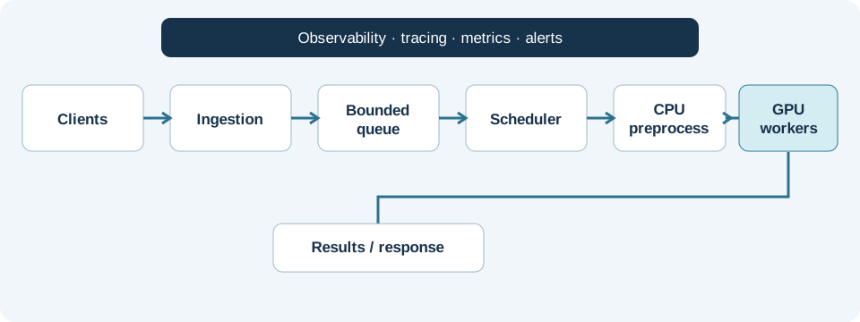
I like to draw this boundary early: ingestion and admission control protect the system; scheduling and workers perform the expensive work; results and telemetry tell us whether the whole path met its contract. The diagram is intentionally simplified, not a depiction of a particular production deployment.
Each stage introduces different constraints. Input decoding may be CPU-bound, data retrieval may be network-bound, and model execution may be limited by GPU compute or memory bandwidth.
Optimizing the model alone doesn’t necessarily improve the end-to-end experience. If requests spend most of their time waiting in a queue, a 20% faster kernel may barely change the latency users see.
2. Choose the right execution model
Synchronous inference is appropriate when clients need immediate responses and execution time is reasonably predictable. Think interactive classification or low-latency APIs.
Asynchronous inference fits longer-running jobs such as video analysis, document processing, or offline batch classification. A queue separates ingestion from execution, allowing the two layers to scale independently.
The trade-off is operational complexity. An asynchronous system needs durable job state, idempotency, retry policies, result storage, and a clear definition of what happens when a worker fails halfway through a job.
My rule is to start with the client’s contract, not a preferred framework. An interactive API needs a clear latency budget. A video-processing job may care more about completion time, durability, and recoverability. The same model can require very different infrastructure depending on that contract.
A synchronous endpoint can still use internal queues and batching. An asynchronous pipeline isn’t automatically reliable just because a message broker is present; it needs explicit ownership of retries, duplicate processing, and result state.
3. Batching: throughput versus latency
GPUs are optimized for parallel computation. Executing every small request independently can leave substantial capacity unused. Batching groups requests into fewer model invocations and may improve throughput.
But the queue is part of latency. A request waiting for a batch to fill is not making progress. Larger batches can improve aggregate efficiency while hurting p95 or p99 latency. That trade-off should be visible, not hidden inside a serving framework.
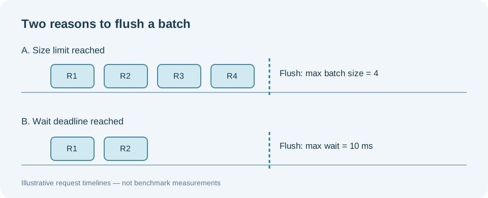
I think of the batcher’s job as enforcing two independent limits: stop waiting when the batch is full, and stop waiting when the oldest request reaches its deadline. Neither limit is a universal constant. Both depend on the traffic pattern and model.
A dynamic batcher typically needs two limits:
- Maximum batch size, bounded by model and GPU memory characteristics.
- Maximum queue wait, bounded by latency objectives.
Input shapes matter too. Padding variable-length sequences to the longest item in a batch can waste compute. Shape-aware grouping can improve efficiency, but excessive grouping can increase wait time for uncommon shapes.
For autoregressive LLMs, continuous batching allows requests to enter and leave the active execution set as tokens are generated. This differs from static batching of one-shot classifiers, and it introduces additional memory and scheduling considerations.
4. Scheduling across distributed workers
A scheduler decides where requests should execute. Simple round-robin routing is easy to implement, but it ignores meaningful differences in worker load.
For example, two GPU workers may have the same hardware but very different effective capacity if one is handling long-running requests.
Useful scheduling signals include queue depth, active requests, estimated work, model availability, accelerator memory, and worker health.
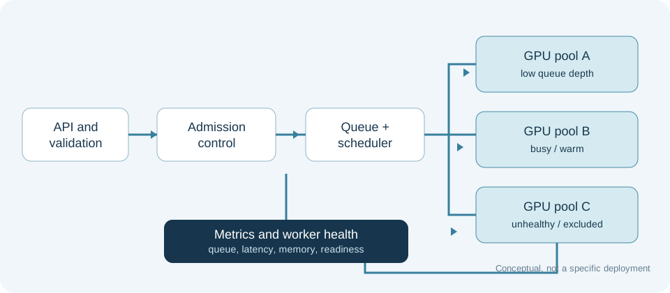
This is where my distributed-systems background influences how I think about inference. I prefer to separate placement from execution: the router makes a decision using imperfect, slightly stale signals; the worker executes and reports what actually happened. That separation makes it easier to reason about retries, health, and overload.
A practical policy might avoid a worker whose model isn’t loaded, reject a worker that is failing readiness checks, and prefer the least-backed-up compatible worker. It still needs guardrails: continuously chasing the lowest queue depth can cause thrashing, and a single long-running request can make simple queue-length comparisons misleading.
Kubernetes can manage deployment, restart unhealthy pods, and scale worker replicas. But the application still needs workload-aware routing, admission control, and sensible overload behavior.
5. Autoscaling is more than GPU utilization
GPU utilization is a useful metric, but it is not a complete demand signal. A heavily queued service can appear healthy while latency deteriorates. Conversely, a GPU may show bursts of high utilization without requiring more replicas.
For many inference services, scaling decisions should combine queue depth, request arrival rate, service time, tail latency, and resource headroom.
New replicas also need time to start, load model weights, and warm up. Scaling policies should account for this delay to avoid reacting too late to demand spikes.
6. Observability: measure the full path
At minimum, instrument the stages that contribute to end-to-end latency:
| Metric | What it tells you |
|---|---|
| End-to-end p50 / p95 / p99 | What clients experience |
| Queue wait time | Whether scheduling or capacity is the bottleneck |
| Preprocessing latency | Whether input handling dominates |
| Model execution latency | How efficiently inference runs |
| Batch size distribution | Whether batching policy matches traffic |
| GPU memory / utilization | Whether resources are constrained or underused |
| Errors, retries, timeouts | Whether the service is stable under load |
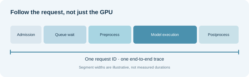
The first dashboard I’d build is an end-to-end latency breakdown, not a GPU utilization chart. I want to know how much time requests spend waiting, preparing, executing, and returning. Traces should connect these stages under a single request or job identifier.
That distinction matters in practice: a faster model won’t fix an overloaded input decoder, and more GPU replicas won’t help if the scheduler is the bottleneck.
7. Reliability is part of performance
When traffic spikes, unbounded queues can create an illusion of availability while response times grow without limit. Bounded queues, backpressure, timeouts, and admission control help protect the service.
Retries require care. Automatically retrying expensive requests during overload can amplify the incident. Asynchronous systems also need idempotent job processing so a retried request doesn’t produce inconsistent results or unnecessary duplicate work.
The goal isn’t merely to keep workers running. It’s to maintain predictable behavior under partial failures and excess demand.
8. What I would benchmark first
Before tuning an inference stack, I would establish a reproducible baseline:
- Choose representative input sizes and traffic patterns.
- Measure throughput and end-to-end latency with batching disabled.
- Sweep batch size and maximum wait time.
- Record GPU utilization, memory use, and queue depth.
- Repeat under bursty traffic and degraded-worker scenarios.
- Compare results against explicit latency and cost objectives.
The results should determine the next optimization. If preprocessing dominates, tuning CUDA kernels is unlikely to be the best first move.
A reproducible policy experiment
I’ve included a small Python batching-policy simulation in the repository. It uses seeded synthetic request arrivals and a configurable service-time curve to compare batch-size and wait-time policies:
python3 examples/inference_benchmark.py --requests 2000 --rate 200 --seed 42It reports simulated p50, p95, and throughput. These are not GPU benchmark results: there is no real model, CUDA execution, network, or Kubernetes scheduler in the experiment. Its value is narrower and more honest—it makes the queueing assumptions visible and gives us a reproducible starting point.
For a real serving benchmark, I’d run the same workload against a deployed model, report hardware and model versions, include warm-up, record the full latency distribution, and publish the raw harness and configuration alongside any charts.
9. A minimal dynamic batching example
The following simplified Python example illustrates the two batching constraints. It’s intentionally a sketch rather than a production-ready server. The separate simulation above is easier to run and compare without installing GPU dependencies:
import asyncio
import time

class DynamicBatcher:
    def __init__(self, infer, max_batch_size=16, max_wait_ms=10):
        self.infer = infer
        self.max_batch_size = max_batch_size
        self.max_wait_s = max_wait_ms / 1000
        self.queue = asyncio.Queue()

    async def submit(self, payload):
        future = asyncio.get_running_loop().create_future()
        await self.queue.put((payload, future))
        return await future

    async def run(self):
        while True:
            first = await self.queue.get()
            batch = [first]
            deadline = time.monotonic() + self.max_wait_s
            while len(batch) < self.max_batch_size:
                remaining = deadline - time.monotonic()
                if remaining <= 0:
                    break
                try:
                    batch.append(await asyncio.wait_for(
                        self.queue.get(), timeout=remaining
                    ))
                except asyncio.TimeoutError:
                    break
            inputs = [item for item, _ in batch]
            try:
                outputs = await self.infer(inputs)
                if len(outputs) != len(batch):
                    raise ValueError("Inference output count mismatch")
                for (_, future), output in zip(batch, outputs):
                    if not future.done():
                        future.set_result(output)
            except Exception as error:
                for _, future in batch:
                    if not future.done():
                        future.set_exception(error)
A real service also needs bounded admission, cancellation handling, shape-aware grouping, worker lifecycle management, instrumentation, and a deliberate overload policy. The infer callback must be asynchronous or offload blocking GPU work so it does not stall the event loop.
Closing thoughts
The lesson I keep coming back to is that inference performance is a property of the whole system. Model speed matters, but so do scheduling, data movement, resource efficiency, observability, and failure behavior.
I don’t think the goal should be the most sophisticated serving stack. I’d rather have a system whose latency budget is explicit, whose overload behavior is predictable, and whose bottlenecks we can explain with evidence. Once those foundations are in place, model-level optimization becomes much more meaningful.
Next in this series: taking this batching policy into a real serving harness, then measuring the throughput–latency trade-off with a documented model and hardware setup.